Kim–Barbulescu variant of the Number Field Sieve to compute discrete logarithms in finite fields

In February 2016, Kim and Barbulescu posted on eprint a merged version of two earlier pre-prints ([eprint:Kim15] and [eprint:Barbulescu15]). This preprint is about computing discrete logarithms (DL) in finite fields and presents a new variant of the Number Field Sieve algorithm (NFS) for finite fields $\mathbb{F}_{p^n}$ . The Number Field Sieve algorithm can be applied to compute discrete logarithms in any finite field of medium to large characteristic $\mathbb{F}_{p^n}$ . Kim and Barbulescu improve its asymptotic complexity for finite fields where $n$ is composite, and one of the factors is of an appropriate size. The paper restricts to non-prime-power extension degree (e.g. $n=9$ or $n=16$ is not targeted) but a generalization to any non-prime $n$ is quite easy to obtain. Typical finite fields that are target groups in pairing-based cryptography are affected, such as $\mathbb{F}_{p^6}$ and $\mathbb{F}_{p^{12}}$ .

Pairing-based cryptography

A pairing is a bilinear map defined over an elliptic curve. It outputs a value in a finite field. This is commonly expressed as 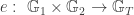$e : ~ \mathbb{G}_1 \times \mathbb{G}_2 \to \mathbb{G}_T$ where $\mathbb{G}_1$ and $\mathbb{G}_2$ are two (distinct) prime order subgroups of an elliptic curve, and $\mathbb{G}_T$ is the target group, of same prime order. More precisely, we have

$\begin{array}{lccccc} e: & \mathbb{G}_1 & \times & \mathbb{G}_2 & \to & \mathbb{G}_T \\ & \cap & & \cap & & \cap \\ & E(\mathbb{F}_p)[\ell] & & E(\mathbb{F}_{p^n})[\ell] & & \boldsymbol{\mu}_{\ell} \subset \mathbb{F}_{p^n}^{*}\\ \end{array}$

where $\boldsymbol{\mu}_{\ell}$ is the cyclotomic subgroup of $\mathbb{F}_{p^n}^{*}$ , i.e. the subgroup of $\ell$ -th roots of unity: $\boldsymbol{\mu}_{\ell} = \left\{ z \in \mathbb{F}_{p^n}^{*}, ~ z ^ \ell = 1 \right\}~.$

The use of pairings as a constructive tool in cryptography had some premices in 1999 and started to be used in 2000. Its security relies on the intractability of the discrete logarithm problem on the elliptic curve (i.e. in $\mathbb{G}_1$ and $\mathbb{G}_2$ ) and in the finite field $\mathbb{F}_{p^n}$ (i.e. in $\mathbb{G}_T$ ).

The expected running-time of a discrete logarithm computation on an elliptic curve and in a finite field is not the same: this is $O(\sqrt{\ell})$ in the group of points $E(\mathbb{F}_p)[\ell]$ , and this is $L_{p^n}[1/3, c]$ in a finite field $\mathbb{F}_{p^n}$ , where $L$ is the notation $L_{p^n}[1/3, c] = \exp\left( (c+o(1)) (\log p^n)^{1/3} (\log \log p^n)^{2/3} \right) ~.$ The asymptotic complexity in the finite field depends on the total size $p^n$ of the finite field. It means that we can do cryptography in an order $\ell$ subgroup of $\mathbb{F}_{p^n}$ , whenever $p^n$ is large enough.

Small, medium and large characteristic.

The finite fields are commonly divided into three cases, depending on the size of the prime $p$ (the finite field characteristic) compared to the extension degree $n$ . Each of the three cases has its own index calculus variant, and the most appropriate variant that applies qualifies the characteristic (as small, large or medium):

small characteristic: one uses the function field sieve (FFS) algorithm, and the quasi-polynomial-time algorithm when the extension degree is suitable for that (i.e. smooth enough);
medium characteristic: one uses the NFS-HD algorithm. This is the High Degree variant of the Number Field Sieve (NFS) algorithm. The elements involved in the relation collection are of higher degree compared to the regular NFS algorithm.
large characteristic: one uses the Number Field Sieve algorithm.

Each variant (QPA, FFS, NFS-HD and NFS) has a different asymptotic complexity.

Quasi Polynomial Time algorithm for small characteristic finite fields

Small characteristic finite fields such as $\mathbb{F}_{2^n}$ and $\mathbb{F}_{3^n}$ where $n$ is composite are broken for pairing-based cryptography with the QPA algorithm (see this blog post).
It does not mean that supersingular curves are broken but it means that the pairing-friendly curves in small characteristic are broken, and only supersingular pairing-friendly curves were available in small characteristic. There exist supersingular pairing-friendly curves in large characteristic which are still safe, if the finite field $\mathbb{F}_{p^n}$ is chosen of large enough size.

How it affects pairing-based cryptography.

It was assumed in order to set up the key-sizes of pairing-based cryptography that computing a discrete logarithm in any finite field $\mathbb{F}_{p^n}$ of medium to large characteristic is of same difficulty at least as computing a discrete logarithm in a prime field of the same total size. The key-size were chosen according to the complexity formula $L_{p^n}[1/3, (64/9)^{1/3} = 1.923]$ .

The finite fields targeted by this new variant are of the form $\mathbb{F}_{p^n}$ , where $n$ is composite (e.g. $n=6$ , $n=12$ ) and there exists a small factor $d$ of $n$ (e.g. 2 or 3 for 6 and 12). In that case, this is possible to consider both the finite field $\mathbb{F}_{p^n}$ and the two number fields involved in the NFS algorithm as a tower of an extension of degree $n/d$ on top of an extension of degree $d$ . With this representation, combined with previously known polynomial selection methods, the norm of the elements involved in the relation collection step (second step of the NFS algorithm) is much smaller. This provides an important speed-up of all the algorithm and decreases the asymptotic complexity below the assumed $L_{p^n}[1/3, 1.92]$ complexity. That is why in certain cases, the key sizes should be enlarged.

Outline

It start with a brief summary on the previous state of the art in DL computation in $\mathbb{F}_{p^n}$ , then the Kim–Barbulescu variant is sketched, and a possible key-size update in pairing-based cryptography is discussed. This is not reasonnable at the time of writting to propose practical key-size update, but we can discuss about an estimate, based on the new asymptotic complexities.

The Number Field Sieve algorithm (NFS)

The NFS algorithm to compute discrete logarithms applies to finite fields $\mathbb{F}_{p^n} = \mathbb{F}_q$ where $p$ (the characteristic) is of medium to large size compared to the total size $p^n$ of the finite field. This is measured asymptotically as $p \geq L_{p^n}[\alpha, c]$ where $\alpha > 1/3$ and the $L$ notation is defined as $L_{p^n}[1/3, c] = \exp\left( (c+o(1)) (\log p^n)^{1/3} (\log \log p^n)^{2/3} \right) ~.$

Since in pairing-based cryptography, small characteristic is restricted to $\mathbb{F}_{2^n}$ and $\mathbb{F}_{3^n}$ , we can simplify the situation and say that the NFS algorithm and its variants apply to all the non-small-characteristic finite fields used in pairing-based cryptography. The Kim–Barbulescu pre-print contains two new asymptotic complexities for computing discrete logarithms in such finite fields. Prime fields $\mathbb{F}_p$ are not affected by this new algorithm. The finite fields used in pairing-based cryptography that are affected are $\mathbb{F}_{p^6}$ and $\mathbb{F}_{p^{12}}$ for example.

The NFS algorithm is made of four steps:

polynomial selection,
relation colection,
linear algebra,
individual discrete logarithm.

The Kim–Barbulescu improvement presents a new polynomial selection that combines the Tower-NFS construction (TNFS) [AC:BarGauKle15] with the Conjugation technique [EC:BGGM15]. This leads to a better asymptotic complexity of the algorithm. The polynomial selection determines the expected running time of the algorithm. The idea of NFS is to work in a number field instead of a finite field, so that a notion of small elements exists as well as a factorization of the elements into prime ideals. This is not possible in a finite field $\mathbb{F}_{p^n}$ .

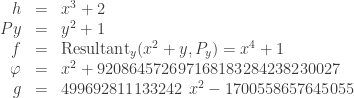
Take as an example the prime $p =$ 3141592653589793238462643383589 $= \lfloor 10^{30}\pi \rfloor + 310$ as in Kim Barbulescu eprint and consider $\mathbb{F}_{p^6}$ . The order of the cyclotomic subgroup is $p^2 - p + 1 = 7\cdot 103 \cdot \ell$ and the 194-bit prime $\ell =$ 13688771707474838583681679614171480268081711303057164980773 is the largest prime divisor of $p^2 - p + 1 = \Phi_6(p)$ . Since $p\equiv 1 \bmod 6$ , one can construct a Kummer extension $\mathbb{F}_p[x]/(x^6+2)$ , where $f(x) = x^6+2$ is irreducible modulo $p$ . Then to run NFS, the idea of Joux, Lercier, Smart and Vercauteren in 2006 [JLSV06] was to use $\mathbb{Z}[x]/(f(x))$ as the first ring, and $\mathbb{Z}[x]/(g(x)$ where $g(x)=f(x)+p$ as the second one to collect relations in NFS. Take the element $971015 \alpha_f^2 + 958931 \alpha_f + 795246$ . Its norm in $\mathbb{Z}[\alpha_f] = \mathbb{Z}[x]/(f(x))$ is 122-bit long. Its norm in $\mathbb{Z}[\alpha_g] = \mathbb{Z}[x]/(g(x))$ is 322-bit long, the total is 444 bits.

Why do we need two sides (the two rings $\mathbb{Z}[x]/(f(x))$ and $\mathbb{Z}[x]/(g(x))$ )? Because when mapping these two elements from $\mathbb{Z}[x]/(f(x))$ and $\mathbb{Z}[x]/(g(x))$ to $\mathbb{F}_{p^n}$ , one maps $x \mapsto z$ since $f \equiv g \bmod p$ , so that $971015 \alpha_f^2 + 958931 \alpha_f + 795246 \mapsto 971015 z^2 + 958931 z + 795246$ and at the same time, $971015 \alpha_g^2 + 958931 \alpha_g + 795246$ is mapped to the same element. What is the purpose of all of this? We will obtain a different factorization into prime ideals in each ring, so that we will get a non-trivial relation when mapping each side to $\mathbb{F}_{p^n}$ . Now the game is to define polynomials $f$ and $g$ such that the norm is as low as possible, so that the probability that an element will factor into small prime ideals is high.

A few new polynomial selection methods were proposed since 2006, to reduce this norm, hence improving the asymptotic complexity of the NFS algorithm. In practice, each finite field is a case study, and the method with the best asymptotic running-time will not obviously gives the smallest norms in practice. That is why cryptanalysts compare the norm bounds in addition to comparing the asymptotic complexity. This is done in Table 5 and Fig. 2 of the Kim–Barbulescu pre-print.

What is the key-idea of the Kim–Barbulescu method? It combines two previous techniques: the Tower-NFS variant [AC:BarGauKle15] and the Conjugation polynomial selection method [EC:BGGM15]. Moreover, it exploits the fact that $n$ is composite. Sarkar and Sigh started in this direction in [EC:SarSin16] and obtained a smaller norm estimate (the asymptotic complexity was not affected significatively). We mention that few days ago, Sarkar and Singh combined the Kim–Barbulescu technique with their polynomial selection method [EPRINT:SarSin16].

Here is a list of the various polynomial selection methods for finite fields $\mathbb{F}_{p^n}$ .

the Joux–Lercier–Smart–Vercauteren method that applies to medium-characteristic finite fields, a.k.a. JLSV1, whose asymptotic complexity is $L_{p^n}[1/3, (128/9)^{1/3} = 2.42]$ .
the Conjugation method that applies to medium-characteristic finite fields, whose asymptotic complexity is $L_{p^n}[1/3, (32/3)^{1/3} = 2.201]$ .
the JLSV2 method that applies to large-characteristic finite fields, whose asymptotic complexity is $L_{p^n}[1/3, (64/9)^{1/3} = 1.923]$ .
the generalized Joux–Lercier (GJL) method that applies to large-characteristic finite fields, whose asymptotic complexity is $L_{p^n}[1/3, (64/9)^{1/3} = 1.923]$ .
the Sarkar–Singh method that allows a trade-off between the GJL and the Conjugation method when $n$ is composite.

Back to our $\mathbb{F}_{p^6}$ example, the Kim–Barbulescu technique would define polynomials such as
$\begin{array}{rcl} h &=& x^3 + 2 \\ Py &=& y^2 + 1 \\ f &=& \mbox{Resultant}_y(x^2 + y, P_y) = x^4 + 1 \\ \varphi &=& x^2 + 920864572697168183284238230027 \\ g &=& 499692811133242\ x^2 - 1700558657645055 \\ \end{array}$
In this case, the elements involved in the relation collection step are of the form $(a_{0}+a_{1}\alpha_h+a_2\alpha_h^2) + (b_0+b_1\alpha_h + b_2\alpha_h)\alpha_f$ . They have six coefficients. in order to enumerate a set of same global size $E^2$ where $E = 2^{30}$ , one takes $\|a_i\|, \|b_i\| \leq E^{2/(t \deg h)} = 2^{10}$ . The norm of $c = ({1018} + {1019} \alpha_h + {1020} \alpha_h^2) + ({1021} + {1022} \alpha_h + {1023} \alpha_h^2) \alpha_f$ is 135.6 bit long, the norm of $d = ({1018} + {1019} \alpha_h + {1020} \alpha_h^2) + ({1021} + {1022} \alpha_h + {1023} \alpha_h^2) \alpha_g$ is 216.6 bit long, for a total of 352.2 bits. This is 92 bits less than the 444 bits obtained with the former JLSV technique.

Why the norm is smaller.

The norm computed in the number fields depends on the coefficient size and the degree of the polynomials defining the number fields, and on the degree and coefficient size of the element whose norm is computed.

With the Kim–Barbulescu technique, the norm is computed recursively from $K_f$ to $K_h$ then from $K_h$ to $\mathbb{Q}$ . The norm formula depends on the degree of the element and since this element is of degree 1 in $K_f$ , its norm will be as low as possible. Then in $K_h$ , the element is of degree (at most) $\deg h -1$ but this does not increase its norm since the coefficients of $h$ are tiny (a norm bound is $A^{\deg h} \|h\|_\infty^{\deg h -1}$ , and $\|h\|_\infty^{\deg h -1}$ will be very small).

Why it changes the asymptotic complexity.

The asymptotic complexity is reduced (contrary to the Sarkar–Singh method) because the norm formula is reduced not only in practice but also in the asymptotic formula. To do so, the parameters should be tuned very tightly. In the large characteristic case, $\kappa = n/\deg h$ should stay quite small: 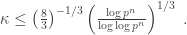$\kappa \leq \left(\frac{8}{3}\right)^{-1/3} \left( \frac{\log p^n}{\log\log p^n} \right)^{1/3}~.$ For $p^n$ of 608 bits as in the $\mathbb{F}_{p^6}$ example, the numerical value is $\kappa \leq 2.967$ . Kim and Barbulescu took $\kappa = 2$ . In fact, $\kappa$ should be as small as possible, so that one can collect relations over elements of any degree in $\alpha_h$ , but always degree 1 in $\alpha_f$ . The smallest possible value is $\kappa = 2$ when $n$ is even.

For the classical BN curve example where $p^{12}$ is a 3072-bit prime power, the bound is $\kappa \leq 4.705$ .

Special-NFS variant when $p$ is given by a polynomial.

For prime fields where $p$ has a special form, the Special-NFS algorithm may apply. Its complexity is $L_{p}[1/3, (32/9)^{1/3} = 1.526]$ . For extension fields $\mathbb{F}_{p^n}$ , where $p$ is obtained by evaluating a polynomial of degree $d$ at a given value, e.g. $d=4$ for BN curves, Joux and Pierrot [PAIRING:JouPie13] proposed a dedicated polynomial selection method such that the NFS algorithm has an exptected running-time of

$L_{p^n}\left[1/3, \left(\frac{d+1}{d}\frac{64}{9}\right)^{1/3}\right]$ in medium characteristic, where $p = L_{p^n}[\alpha_p, c_p]$ and $1/3 < \alpha_p < 2/3$ ;
$L_{p^n}\left[1/3, \left(\frac{32}{9}\right)^{1/3}\right]$ in large characteristic, where $p = L_{p^n}[\alpha_p, c_p]$ and $2/3 < \alpha_p < 1$ and moreover $d$ satisfies $d = \frac{1}{n} \left(\frac{2 \log p^n}{3 \log \log p^n} \right)^{1/3}$ ;
$L_{p^n}\left[1/3, \left(\frac{32}{9}\right)^{1/3}\right]$ in prime fields and tiny extension degree fields, where $p = L_{p^n}[1, c_p]$ and moreover $d$ satisfies $d = \frac{1}{n} \left(\frac{2 \log p^n}{3 \log \log p^n} \right)^{1/3}$ .

The Kim–barbulescu method combines the TNFS method and the Joux–Pierrot method to obtain a $L_{p^n}[1/3, (32/9)^{1/3} = 1.526]$ asymptotic complexity in the medium-characteristic case.

Discussion on key-size update

This new attack reduces the asymptotic complexity of the NFS algorithm to compute DL in $\mathbb{F}_{p^n}$ , which contains the target group of pairings. The recommended sizes of $\mathbb{F}_{p^n}$ were computed assuming that the asymptotic complexity is $L_{p^n}[1/3, 1.923]$ . Since the new complexity is below this bound, the key sizes should be enlarged. The smallest asymptotic complexity that Kim and Barbulescu obtain is for a combination of Extended-TNFS and Special-NFS. They obtain $L_{p^n}[1/3, (32/9)^{1/3} = 1.526]$ when the prime $p$ is given by a polynomial of degree $d$ and when $n$ is composite, $n=\kappa \eta$ , and $\eta$ satisfies an appropriate bound. In that case, it means that the size of $\mathbb{F}_{p^n}$ should be roughly doubled asymptotically.

Comparison with NFS in prime fields $\mathbb{F}_{p_1}$ .

In order to provide a first comparison of the expected running-time of the NFS algorithm in finite fields $\mathbb{F}_{p^n}$ and prime fields $\mathbb{F}_{p_1}$ of same total size, one can compare the size of the norms involved in the relation collection. We took the $\mathbb{F}_{p^6}$ example of 608 bits (183 decimal digits), and consider a prime field of 608 bits for comparison. The Joux–Lercier method [MathComp:JouLer03] generates two polynomials $f$ and $g$ of degree $d+1$ and $d$ and coefficient size $\| f \|_\infty = O(1)$ , $\| g \|_\infty = O(p^{1/(d+1)})$ . We take $d \approx \delta \left( \frac{\log p}{\log \log p} \right)^{1/3}$ , where $\delta = 3^{1/3}/2$ . We obtain $d = 2.95$ . We take $d=2$ . The choice $d=3$ would end to slightly larger norms (5 to 10 bit larger).
The polynomials $f$ and $g$ would be of degree 3 and 2, and the coefficient size of $g$ would be $p^{1/3}$ of 203 bits. The bound $E$ in the relation collection would be approximately $\log_2 E \approx 1.1 (\log q)^{1/3} (\log \log q)^{2/3}$ (in theory $L_p[1/3, \beta=(8/9)^{1/3}]$ ) of 27.36 bits (cado-nfs) up to 30 bits (Kim–Barbulescu estimate). The norms of the elements would be $d^2 E^{2d+1} p^{1/(d+1)}$ of 341 bits ( $\log_2 E = 27.36$ ) to 354 bits ( $\log_2 E = 30$ ). Kim and Barbulescu obtain a norm of 330 bits for $\mathbb{F}_{p^6}$ [Example 1]. It means that computing a discrete logarithm in $\mathbb{F}_{p^6}$ compared to $\mathbb{F}_{p_1}$ both of 608 bits would be easier in $\mathbb{F}_{p^6}$ .

We can do the same analysis for $\mathbb{F}_{p^{12}}$ of 3072 bits and this starts to be a complete mess. The Joux–Lercier method for a prime field $\mathbb{F}_{p1}$ of 3072 bits would take polynomials of degree $d=4$ and the norms would be of 1243 bits. The Kim–Barbulescu technique (ExTNFS) with Conjugation in $\mathbb{F}_{p^{12}}$ of 3072 bits would involve norms of 696 bits in average. If moreover we consider a BN-prime given by a polynomial of degree 4, and take $\eta=3$ and $\kappa = 4$ , the norms would be of 713 bits in average. This is also what [Fig. 3] shows: the cross-over point betweeen ExTNFS-Conj (of asymptotic complexity $L_{p^n}[1/3, 1.92]$ ) and Special ExTNFS (of asymptotic complexity $L_{p^n}[1/3, 1.52]$ ) is above 4250 bits.

Security level estimates and key-sizes.

[Edited May 3 thanks to P.S.L.M. B. comments]
What would be the actual security level of a BN curve with $p$ of 256 bits and $\mathbb{F}_{p^{12}}$ of 3072 bits? At the moment, the best attack would use a combination of Extended TNFS with the Joux–Pierrot polynomial selection for special primes, or the ExTNFS with Conjugation. We give in the following table a rough estimate of the improvement. Evaluating the asymptotic complexity $L_{p^n}[1/3, c]$ for a given finite field size does no provide the number of bits of security but could give a (theoretical) hint on the improvements of the Kim–Barbulescu technique. This table can only say that the former 256-bit prime $p$ BN curve should be changed into a 448 up to 512-bit prime $p$ BN-curve.
This is a rough and theoretical estimate. This can only says that a new low bound on the size of BN-like $\mathbb{F}_{p^{12}}$ to achieve a 128-bit security level would be at least 5376 bits ( $p$ of 448 bits).

[edited June 8th thanks to T. Kim comments. In the medium prime case, the best complexity of Extended TNFS is $L_{p^n}[1/3, 1.74]$ when $n$ is composite. ]
$\begin{array}{|c|c|c|c|c|c|c|} \hline \log_2 p & n & \log_2 q & \begin{array}{@{}c@{}} \mbox{Joux--Pierrot NFS}\\ d=4, L_{p^n}[1/3, 2.07] \end{array} & \begin{array}{@{}c@{}} \\ L_{p^n}[1/3, 1.92] \end{array} & \begin{array}{@{}c@{}} \mbox{Extended TNFS}\\ L_{p^n}[1/3, 1.74] \end{array} & \begin{array}{@{}c@{}} \mbox{Special Extended TNFS}\\ L_{p^n}[1/3, 1.53] \end{array} \\ \hline 256 & 12 & 3072 & \approx 2^{149-\delta_1} & \approx 2^{139-\delta_2} & \approx 2^{126-\delta_3} & \approx 2^{110-\delta_4} \\ \hline 384 & 12 & 4608 & \approx 2^{177-\delta_1} & \approx 2^{164-\delta_2} & \approx 2^{149-\delta_3} & \approx 2^{130-\delta_4} \\ \hline 448 & 12 & 5376 & \approx 2^{189-\delta_1} & \approx 2^{175-\delta_2} & \approx 2^{159-\delta_3} & \approx 2^{139-\delta_4} \\ \hline 512 & 12 & 6144 & \approx 2^{199-\delta_1} & \approx 2^{185-\delta_2} & \approx 2^{168-\delta_3} & \approx 2^{147-\delta_4} \\ \hline \end{array}$

To obtain a key size according to a security level, a value $\delta_i$ is required, which is not known. The order of magnitude of this $\delta_i$ is usually of a dozen. A 4608-bit field (corresponding for Barreto-Naehrig curves to $p$ of 384 bits) might not be large enough to achieve a 128-bit security level.

Alternative choices of pairing-friendly curves.

Few days ago, Chatterjee, Menezes and Rodriguez-Henriquez proposed to use embedding degree one curves as a safe alternative for pairing-based cryptography. However in these constructions, the prime $p$ is given by a polynomial of degree 2. It is not known what is the most secure: a prime field with $p$ given by a polynomial of degree 2 or a supersingular curve with $k=2$ (or even a MNT curve with $k=3$ ).

Another way would be to use generic curves of embedding degree $n=2$ or $n=3$ , generated with the Cocks-Pinch method, so that no one of the recent attacks can apply. In any case the pairing computation would be much less efficient than previously with the BN curves and $p$ of 256 bits. Such low embedding degree curves were used at the beginning of pairing implementation, e.g. [CT-RSA:Scott05], [ICISC:ChaSarBar04].

Aurore Guillevic.

12 Responses to Kim–Barbulescu variant of the Number Field Sieve to compute discrete logarithms in finite fields

I'm the B in "BN curves" says:

May 3, 2016 at 5:48 am

I think there are some typos around the paragraph that reads “This is a rough and theoretical estimate.” The table (which I checked) indicates that 128-bit security needs 384 bits BN curves, not 448 or 512. Also, the text there sounds a little strange (copy&paste&modify from previous paragraph, maybe?)

Aurore Guillevic says:

May 3, 2016 at 2:47 pm

This is not easy to extrapolate key-sizes according to an asymptotic formula. The main issue with the NFS-like asymptotic formulas is the $o(1)$ in the exponent, that hides all the polynomial factors. That is why this is not enough to compute a key-size only according to a formula such as $L_{p^n}[1/3, c]$ .
To estimate a key size, we need the asymptotic formula $L_{p^n}[1/3, c]$ and a constant obtained by a real-life computational record, to calibrate the asymptotic formula. This can be done for prime fields:
The last DL record computation in a prime field was in 2014, in a 595-bit prime field.
[BGIJT14]

Assuming that the computational effort was of approximately $2^{65}$ , we can calibrate the asymptotic formula accordingly. The asymptotic complexity is $L_{p}[1/3, (64/9)^(1/3)]$ . One needs to find a constant $C$ such that $C L_{p}[1/3, (64/9)^(1/3)] = 2^{65}$ where $\log_2 p = 596$ bits. This is $C = -3.4$ . Then an extrapolation is possible.

There is no such real-life record computation available to calibrate the asymptotic formula of the new Kim–Barbulescu paper, and that is why a tight recommendation is not given.

- Aurore Guillevic says:
  
  May 4, 2016 at 4:06 pm
  
  Of course this is $C = 2^{-3.4}$ .
  
I'm the B in "BN curves" says:

May 3, 2016 at 8:01 pm

What I’m saying is that your *text* claims 448-bit curves for 128-bit security, yet your *table* reports ~130-bit security for 384-bit curves.

Aurore Guillevic says:

May 3, 2016 at 10:02 pm

This is too early to claim any key size for a given security level. We really need a record computation.
The table was edited. Thanks.

daira says:

May 17, 2016 at 12:43 pm

“The asymptotic complexity is reduced (contrary to the Sarkar–Singh method) because the norm formula is reduced not only in practice but also in the asymptotic formula.”

It may be worth clarifying that this is “contrary to” the original Sarkar–Singh method. If I understand correctly, the Sarkar–Singh method combined with Kim–Barbulescu does give an asymptotic improvement, and is currently the best algorithm. (I’m assuming it can be applied to the “special extended” case as well.)

Zcash (https://z.cash) had been planning to use a BN128 curve, and we’re currently trying to reassess what curve we will need in light of this attack: https://github.com/zcash/zcash/issues/714

ARIEL GABIZON says:

November 30, 2016 at 5:24 pm

Besides asymptotic complexity are the concrete constants in these algorithms small? Are there experimental results? e.g. what is the largest p such that someone has found a DL in F_p^12?

- ellipticnews says:
  
  December 1, 2016 at 2:47 am
  
  There is a lot more discussion about the practical impact of these results in the recent paper “Challenges with Assessing the Impact of NFS Advances on the Security of Pairing-based Cryptography” by Alfred Menezes, Palash Sarkar and Shashank Singh.
  
  http://eprint.iacr.org/2016/1102
  
  - ARIEL GABIZON says:
    
    December 1, 2016 at 8:28 pm
    
    Thanks for that great pointer! Perhaps you could help me.
    I’m looking at Table 4, and it talks about the num of bits p needs for a certain security level with or without ignoring constants.
    For example it says for BN curves with n=12, when not ignoring constants, 256 bits in p is enough for 128 bit security.
    Isn’t *that* the relevant number?
    Why also write the number that ignores the constants?
Pingback: Technical developments in Cryptography: 2016 in Review ~ MCJ™
Palash Sarkar says:

December 27, 2016 at 4:45 pm

The estimates without the constants should be considered to be conservative estimates. See the first paragraph of Section 6.3 of our updated paper at http://eprint.iacr.org/2016/1102.

Pingback: Recent work on pairing inversion | ellipticnews

	Aurore Guillevic on CRYPTO 2020
	Francisco Rodriguez… on Eurocrypt 2020
	Luca De Feo on Isogeny crypto
	Recent work on pairi… on Kim–Barbulescu variant o…
	ellipticnews on Isogeny-based post-quantum cry…